Pipeline Stress Test Simulation Under Freeze-Thaw Cycling via the XGBoost-Based Prediction Model

Introduction

Buried oil and gas transportation plays an important role in the global energy supply. Long-distance oil transportation via buried pipelines often crosses seasonal frozen soil areas, which freeze-thaw cycles induce cyclic stresses in pipelines’ metal. Therefore, the effects of temperature and the number of freeze-thaw cycles on the pipeline stressed state should be analyzed.

Periodic temperature changes often hinder the normal operation of pipelines. In winter, the oil viscosity increases, the paraffin at the bottom of the pipeline accumulates, hindering the oil transportation. Moreover, the pipeline is arched by the freeze-thaw cycle load, resulting in uneven stress on the oil pipeline. Pores are formed between the pipe and the soil, and the pipeline may be broken by additional stresses (Boguchevskaya et al., 2016; Wu et al., 2010). The generation of soil frost heave force is aggravated by high moisture content (Jin et al., 2010; Li et al., 2010; Liu et al., 2014; Dvoskina et al., 2015). The above problems concern all buried oil pipelines that pass through seasonally frozen soil areas.

In gas pipelines, a similar phenomenon is related to the Archimedean force of the water-bearing soil acting on the pipeline (Teng et al., 2021; Mukhametdinov, 1996). Besides, strain accumulation or the so-called ratcheting effect is intrinsic to melting soil-pipeline engineering. This effect increases stresses and displacements of buried oil pipelines with the number of freeze-thaw cycles in seasonal frozen soil areas. As the number of loading cycles increases, this phenomenon mainly manifests itself by increased displacements, which tend to be stable after reaching the maximum value. This displacement accumulation should also be considered in the power engineering, chemical engineering, and metallurgical industries (Gokhfeld and Charniavsky, 1980; Fuschi et al., 2015).

In a freeze-thaw process, the volumetric strain of the water-containing frozen soil is relatively small, so that a significant strain level can be reached only when the pipe strain is accumulated cycle by cycle. The pipeline strain accumulation is restrained by residual stress during inelastic deformation. However, due to the unique plastic deformation of steel, a delay (lag) between the maximum stress and plastic deformation may occur. For the study of stress accumulation in buried pipelines, some scholars have carried out numerical analyses of water-heat coupling (Kang et al., 2016; Zhang et al., 2020a, Zhang et al., 2021 T.) and stress field calculation (Wen et al., 2010).

However, variations of atmospheric temperature, soil moisture content, and soil types along the buried oil pipeline are complex. The heat conduction/convection of pipe soil is often affected by the migration of moisture and the formation of ice lenses (Li et al., 2019). Uneven frost heave, thawing settlement, and pipe warping are very serious pipe-soil disasters (Andersland and Ladanyi, 2003). To study the mechanical evolution of buried oil pipelines, some scholars have carried out frost heaving tests (Slusarchuk et al., 1978; Carlson and Nixon, 1988; Huang et al., 2015; Kim et al., 2008; Xu et al. ., 2010; Huang et al., 2004). Their results indicated a close relationship between the steel grade of the pipe, growth of the elliptical frozen soil area around the pipe sections, frost heave rate, types of soil in different pipe sections, and growing overburden pressure.

The thermal-hydro-mechanical (THM) model can more accurately simulate and predict the frost heaving force, pipeline displacement, and moisture migration of buried pipelines (Nishimura et al. ., 2009; Zhang and Michalowski, 2015; Bekele et al. ., 2017; Haxaire et al., 2017). The operation and maintenance of buried pipelines are affected by surrounding soil temperature, moisture content, frost heave strength, tensile strength, creep, soil elastic modulus, pipeline displacement, buried depth, and steel pipe parameters (Nixon et al., 2016). It is extremely important to predict the stresses and displacements of buried pipelines under freeze-thaw cycles to ensure their safety, stability, and economic benefit. However, the effect of multiple freeze-thaw cycles has not been clarified yet, and only the stress response of the pipeline under a single freeze-thaw cyclic load has been studied in detail. Therefore, the THM coupling model and the respective software package are required to numerically simulate and verify oil pipelines’ stress evolution effectively. The stress evolution of buried pipelines is closely related to the moisture content of surrounding soil, so it is of great significance to study the effect of different moisture contents on pipeline’s stress.

In recent years, machine learning (ML), which could comprehensively learn potential correlations of input and output variables, has been widely applied to nonlinear multi-parameter regression problems (Prayogo et al., 2020). Thus, Xu et al. (2021) combined the XGBoost (an optimized distributed gradient boosting library designed to be highly efficient, flexible, and portable), backpropagation (BP) neural network, and linear regression method to establish a dam deformation prediction model. They concluded that it was problematic to accurately predict the peak of training samples by the tree algorithm. Based on the hybrid method of genetic algorithm and machine learning, Zhang, 2017 extracted the stress analysis characteristics of the plate and predicted the defects. The tree algorithm integrated with the XGBoost (Chen and Guestrin, 2016; Abbasi et al., 2019; Dong et al., 2020; Kim et al., 2020) was introduced into the regularization parameter, effectively avoiding the over-fitting phenomenon. The superposition of numerous decision trees improved the calculation accuracy, while the iterative efficiency was enhanced by the second-order Taylor expansion of the objective function. Given the nonlinear relationship between pipeline stress and atmospheric temperature, soil moisture content, freeze-thaw cycles, and other factors, it is expedient to apply the ML approach to buried oil pipelines.

Stress monitoring of buried oil pipelines under freeze-thaw cycles is hindered by long periods, large data volume, long-distance transmission, and difficulty in installing strain gauges. The XGBoost-based regression can better adapt to the engineering requirements of long periods, high precision, and large oil pipeline stress monitoring data volume. Due to its easy convergence and high fitting prediction accuracy, it has been applied to many fields. However, to the best of the authors’ knowledge, its application to pipeline safety assessment has not been reported yet. This study aimed to fill this gap by predicting the stressed state of a buried pipeline made from the Q345 steel under numerous freeze-thaw cycles. Eleven regression models based on XGBoost and machine learning were realized. The optimal model for the pipeline stress evolution prediction was finally selected by comparing their MSE, MAE, and R² parameters. It furnishes a novel method for stress analysis of pipelines subjected to freeze-thaw cycles.

Principal Analysis

Stress Calculation Formula

The experimental strains measured on the pipeline surface by strain rosettes were monitored as tensile (${\epsilon }_x$ and ${\epsilon }_y$) and shear (${\gamma }_{xy}$) components for the two-dimensional stressed state. These strain components were processed by the strain-processing method proposed by Zhang (2006) as follows:

${\epsilon }_1=\frac{{\epsilon }_x+{\epsilon }_y}{2}+\frac{{\epsilon }_x-{\epsilon }_y}{2}=\frac{1}{2}\left[\left({\epsilon }_0+{\epsilon }_{90}\right)+\sqrt{2\left[{\left({\epsilon }_0-{\epsilon }_{45}\right)}^2+{\left({\epsilon }_{45}-{\epsilon }_{90}\right)}^2\right]}\right](1)$

${\epsilon }_2=\frac{{\epsilon }_x+{\epsilon }_y}{2}+\frac{{\gamma }_{xy}}{2}=\frac{1}{2}\left[\left({\epsilon }_0+{\epsilon }_{90}\right)-\sqrt{2\left[{\left({\epsilon }_0-{\epsilon }_{45}\right)}^2+{\left({\epsilon }_{45}-{\epsilon }_{90}\right)}^2\right]}\right](2)$

where subscripts 0, 45, and 90 correspond to the respective angle θ values.

According to the generalized Hooke’s law

${\sigma }_1=\frac{E}{1-v}\left({\epsilon }_1+v{\epsilon }_2\right)(3)$

${\sigma }_2=\frac{E}{1-v}\left({\epsilon }_2+v{\epsilon }_1\right)(4)$

where E and υ are the material’s elastic modulus and Poisson’s ratio, respectively.

Substituting Eqs 1, 2 into Eqs 3, 4, the first and second principal stresses can be obtained as follows:

${\sigma }_1=\frac{E}{2}\left[\frac{1+v}{1-v}\left({\epsilon }_0+{\epsilon }_{90}\right)+\sqrt{2}\sqrt{{\left({\epsilon }_0-{\epsilon }_{45}\right)}^2+{\left({\epsilon }_{45}-{\epsilon }_{90}\right)}^2}\right](5)$

${\sigma }_2=\frac{E}{2}\left[\frac{1+v}{1-v}\left({\epsilon }_0+{\epsilon }_{90}\right)-\sqrt{2}\sqrt{{\left({\epsilon }_0-{\epsilon }_{45}\right)}^2+{\left({\epsilon }_{45}-{\epsilon }_{90}\right)}^2}\right](6)$

Elaboration of the Principal Stress Prediction Based on XGBoost Algorithm

The XGBoost optimization model with the characteristics of both linear and tree models has been introduced by Chen et al. (2016). By constructing multiple trees to fit the residuals, the model prediction values of all decision trees were accumulated into the final one, and the model was trained by the gradient boosting decision tree (GBDT) algorithm.

In the current elaboration of principal stress prediction models for the Q345 steel pipe, the XGBoost algorithm dealt with the stress prediction function, and new functions of each factor were continuously added to approximate the measured stress values, namely:

${\widehat{y}}_K={\displaystyle \sum _{i=1}^K{F}_i}\left(x_i\right)=F_{K-1}\left(x_i\right)+f\left(T_i+t_i+{\sigma }_1\right)(7)$

where K is the prediction round; ${\widehat{y}}_K$ is the value of the K-th round deformation predictive function; $F_{K-1}\left(x_i\right)$ is the value of the (K-1)th round deformation predictive function; $f\left(T_i+t_i+{\sigma }_1\right)$ is the decision tree function of the temperature factor (T_i) aging factor (t_i), and stress factor (σ₁).

The XGBoost algorithm objective function can be derived by Chen et al. (2016) as follows:

$F_0={\displaystyle \sum _{i=1}^{K}L}\left(y_i,{\widehat{y}}_i\right)+{\displaystyle \sum _{i=1}^K\mathrm{\Omega }}\left(f_K\right)(8)$

where L is the loss function used to evaluate the loss between the predicted and true strain values; $\mathrm{\Omega }\left(f_K\right)$ is a regularization function to control model complexity and avoid overfitting. The regularization function can be defined as follows:

$\mathrm{\Omega }\left(f\right)=\gamma T+\frac{1}{2}\lambda {\Vert \omega \Vert }^2(9)$

where $\gamma$ and $\lambda$ are the penalty coefficients of the regularization item; $\omega$ is the leaf node-corresponding weight; T is the temperature.

By re-arranging (7) and applying the second-order Taylor expansion, we get:

$F_{OK}={\displaystyle \sum _{i=1}^{n}L\left(y_i,{\widehat{y}}_{i,K-1}+f_K\left(x_i\right)\right)}+\mathrm{\Omega }\left(f_K\right)(10)$

$f\left(x+\mathrm{\Delta }x\right)\cong f\left(x\right)+f^{\prime }\left(x\right)\Delta x+\frac{1}{2}{f}^{\prime \prime }\left(x\right)\mathrm{\Delta }{x}^2(11)$

Formula (10) can be further reduced to the following form:

$F_{OK}={\displaystyle \sum _{i=1}^n\left[g_i{f}_K\left(x_i\right)+\frac{1}{2}{h}_i{f}_K^2\left(x_i\right)\right]}+\mathrm{\Omega }\left(f_K\right)(12)$

where $g_i$ and $h_i$ are the loss function’s first- and second-order gradient statistics, respectively. The model training was completed by iteratively finding $f\left(x\right)$ to minimize the objective function.

Time Scaling Principle of Freeze-Thaw Cycles

Since the time and space scales of the heat transfer problem in buried oil pipelines are very large, a reduced similarity ratio was used for the experiment.

According to the similarity theory (Guo et al., 2010), the similarity criterion number of the model was derived as follows:

$F_o=\frac{a{L}_o^2}{\mathrm{\Gamma }}(13)$

where L₀ is characteristic length, m; $\mathrm{\Gamma }$ is the period of surface temperature change, h.

The physical analog properties of the experimental and actual systems were guaranteed. The experiment lasted for 10 days, and the 10-year variation process of the buried pipeline in the existing system under the freeze-thaw cycles’ action was simulated. The specific similarity process is described in Table 1.

TABLE 1

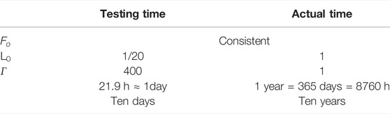
TABLE 1. Actual/testing time conversion.

Taking the Da-Qing section of the China-Russia buried oil pipeline as a reference, a 1:10 downscaled physical analog model of the buried oil pipeline was designed. The specific parameters of the pipeline and model are listed in Table 2.

TABLE 2

TABLE 2. Specific parameters of the pipeline and physical analog model.

TABLE 3

TABLE 3. Evaluation of prediction accuracy (RMSE).

Test and Model Verification

Test Principle and Results

The strain-monitoring data of the performed freeze-thaw cyclic tests with ten cycles were obtained. The specific freeze-thaw test principle is shown in Figure 1, while the actual test box layout is depicted in Figure 2.

FIGURE 1

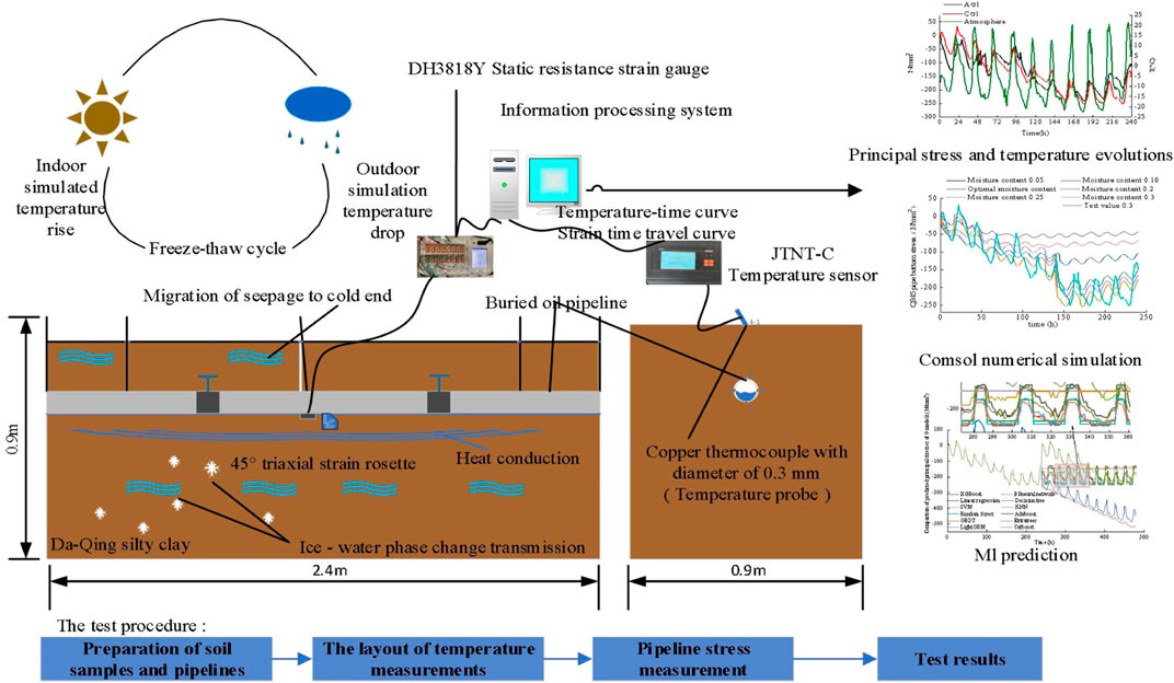
FIGURE 1. Schematic diagram of the test procedure.

FIGURE 2

FIGURE 2. The test box layout.

To explore the effects of temperature and time on the stress at the pipeline bottom, the respective temperature and stress time history curves were plotted, as shown in Figure 3, according to the strain data obtained from the test and calculated via Eqs 5, 6.

FIGURE 3

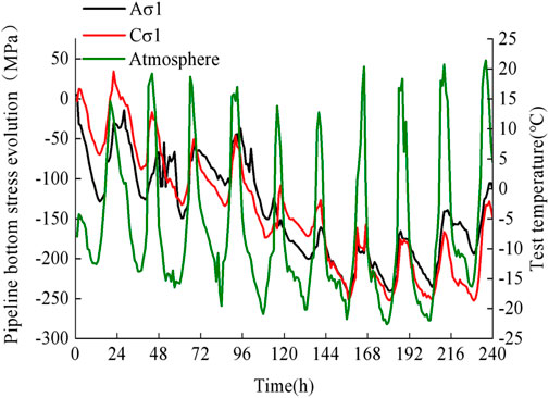
FIGURE 3. Principal stress and temperature evolutions at the pipeline top (Aσ₁) and bottom (Cσ₁).

As shown in Figure 3, the maximum compressive stress at the pipeline bottom was −252.437 MPa, corresponding to 73.17% of the yield stress. It can be seen that the thermal (temperature-induced) stresses strongly impacted the pipeline, which top and bottom were both compressed. This occurred due to a large stiffness of the Q345 steel pipe and the coupled effects of upper soil gravity, pipeline’s and internal fluid’s gravity, and frost heave pressure.

The compressive stress value gradually accumulated and increased with the number of freeze-thaw cycles. After reaching the extreme value after seven or eight freeze-thaw cycles, there was a recovery trend, with a final stabilization. This was consistent with the “ratcheting effect” predicted by the freeze-thaw cycle theory.

The analysis of plots in Figure 3 revealed that the extreme stress at the bottom of the pipeline always occurred 1–2 h after the extreme negative temperature was observed. This finding was consistent with the limit analysis results of Cherniavsky, 2018 for structures subjected to thermal cycling.

COMSOL Simulation Verification

COMSOL modeling process is shown in Figure 4. In seasonally frozen soil areas, the temperature field around the buried oil pipeline is controlled by its thermal properties, the oil temperature in the pipeline, and the number of freeze-thaw cycles. According to the basic theories of heat transfer and frozen soil mechanics, the transient heat conduction equation considering the volumetric strain effect on the temperature fluctuation has the following form:

$C{\rho }_s\frac{\partial T}{\partial t}=div\left(\lambda grad\overrightarrow{T}\right)-L{\rho }_w\frac{\partial {\theta }_w}{\partial y}+{\beta }_{t}T\frac{\partial {\epsilon }_v}{\partial t}(14)$

where C is the specific heat capacity of the frozen soil (J/(kg·°C)); ρ_s and ρ_w are soil and water densities, respectively (kg/m³); λ(θ) is the soil thermal conductivity (W/(m·°C)); L is the latent heat of ice-water phase change in the frozen soil (J/kg); β_t is the thermal stress coefficient of the frozen soil (MPa/K); ε_v is the volumetric strain.

FIGURE 4

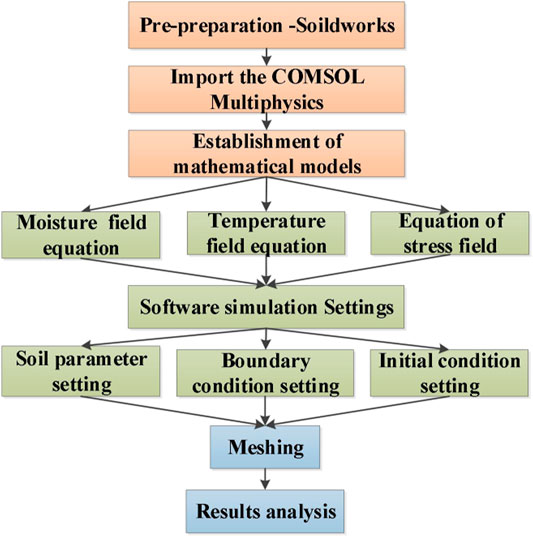
FIGURE 4. The simulation process.

Boundary Conditions

1) Atmospheric temperature at the top of the pipeline was derived as follows:

$T=0.3+24\sin \left(\frac{2\pi }{365}t+\pi \right)(15)$

The boundary conditions on the left and right sides of the pipeline were set as the adiabatic (zero flux) conditions; according to the field drilling data. Finally, the temperature at the bottom of the model was assumed to be unchanged, that is T_CD = -0.89 °C.

$\left|x\right|=l:{\frac{\partial T}{\partial x}|}_{\left|x\right|=l}=0(16)$

$y=-h:{T_s|}_{\left|x\right|=l}=T_{CD}(17)$

2) Boundary conditions for the inner wall temperature of the pipeline were derived as follows. According to the design oil temperature of the China-Russia oil pipeline, the temperature in the pipeline had the following form:

$T=2+8\sin \left(\frac{2\pi }{T_t}t\right)(18)$

3) Boundary conditions of the water field

In the initial conditions of the water field, the initial water content of silty clay was set to 0.3. The pipeline material implied a moisture content of 0, and the water flux of all external boundaries in the calculation was zero.

4) Stress boundary conditions were as follows

$\left|x\right|=l,{\tau }_{xy}=0;y=-h,{\sigma }_x=0(19)$

5) Displacement boundary conditions were:

$\left|x\right|=l,u=0;y=-h,v=0(20)$

Results and Analysis

The temperature, moisture, and pipeline-soil coupled stress fields after ten freeze-thaw cycles were numerically simulated, as shown in Figure 5.

FIGURE 5

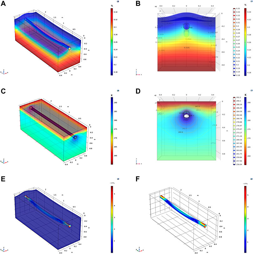
FIGURE 5. Moisture, temperature, and pipe-soil stress fields under freeze-thaw cycles. (A) Moisture field; (B) Moisture field profile; (C) Temperature field; (D) Temperature profile; (E) Pipe-soil stress field; (F) Pipeline stress field.

The COMSOL-based numerical simulation was carried out to explore the initial moisture content effect on the stressed state of the Q345 steel pipeline bottom. The obtained stress evolution curve is presented in Figure 6.

FIGURE 6

FIGURE 6. Stress evolution at the pipeline bottom for various initial moisture contents.

It can be seen in Figure 6 that at the initial moisture content of 0.3, the maximum stress evolution patterns at the pipeline bottom obtained experimentally and via the numerical simulation were consistent, which verified the COMSOL model feasibility. As the moisture content increased, the stresses generated in the pipeline also grew because the soil with high moisture content produced higher frost heave forces during the freeze-thaw cycle.

It can be seen in Figure 6 that the pipe-soil interaction stress increased with the moisture content w, reaching its maximum at 20% < w<30%. This implied that small moisture contents, in particular, the optimal moisture content of 0.16%, slightly affected the frost heave force of the frozen silty clay.

As the moisture content w continued to increase, the soil porosity dropped, promoting the interaction between soil particles. In addition, the water froze into ice, and the ice lens enhanced the pipe-soil bonding force. The stresses at the pipeline bottom increased after the seventh freeze-thaw cycle. Subsequently, the soil pores grew and became saturated, the soil-induced forces were reduced, in contrast to ice-induced ones. The pipeline stress field stabilized, exhibiting a recovery trend.

XGBoost Verification and Comparison With Other ML Algorithms

XGBoost-Based Prediction Procedure

Step 1. The data on the temperature and time-effect factors were processed, and the relevant influencing factor was sorted as the input sample set, which was subdivided into the training set, verification set, test set 1, and test set 2. The verification set was separated from the training set by the cross-validation function.

Step 2. The training and validation sets were sorted and completed; the evaluation index CV was generated by cross-validation. The optimization range of each parameter was determined, and the Bayesian optimization algorithm was brought into the black box non-derivative global optimization. To avoid the local optimum and the predicted value mutation, the parameter group with CV < 0.2 was selected to construct the prediction model, and the training set 1 was predicted. If the predicted value mutation occurred in the selected parameter group, the CV threshold was increased. The training speed and prediction accuracy of each model of each parameter group were comprehensively evaluated. The optimal parameter group and the optimal models were selected to construct the pipeline stress prediction model.

Step 3. The data of test set 2 were incorporated into the model constructed in Step 2 for the model evaluation. The XGBoost model feasibility was evaluated by its comparison with the model based on the LightGBM algorithm (Xu et al., 2021). The respective flowchart is depicted in Figure 7 (Su et al., 2016; Xu et al., 2021).Four kinds of ML regression algorithms, namely the support vector machine (SVM), Random Forest, LightGBM, and XGBoost, were realized, yielding the pipeline bottom stress regression values. These were plotted versus the experimental ones in Figure 8.It can be seen in Figure 8 that each of these 4 ML models achieved high accuracy. Under freeze-thaw cycles, the SVM-predicted stresses at the bottom of the Q345 pipeline ranged from -148.451 to -145.852 MPa. There was a large discrepancy with the experimental value caused by the sensitivity of SVM regression to the selection of parameter adjustment and sum function. Therefore, SVM regression was a poor choice for the prediction model of principal stresses at the top and bottom of the Q345 steel pipe.The maximum relative error was minimized by comparing the predicted and test values, verifying the model’s accuracy. RMSE is an important indicator to evaluate the accuracy of the model and is given in Table 3.It can be seen from Figure 9 that the XGBoost algorithm provided the best prediction of the principal stress at the pipeline bottom for each freeze-thaw cycle. The correlation coefficient was R² = 0.978, the fitting effect was excellent, and the convergence speed was high.The determination coefficients of SVM, Random Forest, and LightGBM models also met the engineering requirements, and the complex local stress was predicted quite accurately. For the XGBoost model, regularization 2 was introduced, and appropriate parameters were adjusted to avoid large overfitting. XGBoost model had a high correlation coefficient R² and low MSE = 0.02, RMSE = 11.07, and MAE = 0.1017. The results showed that under freeze-thaw cycling, the XGBoost model for the bottom stress of the Q345 pipeline had the highest evaluation index, and the model outperformed the other three.

FIGURE 7

FIGURE 7. Modeling process based on the XGBoost algorithm.

FIGURE 8

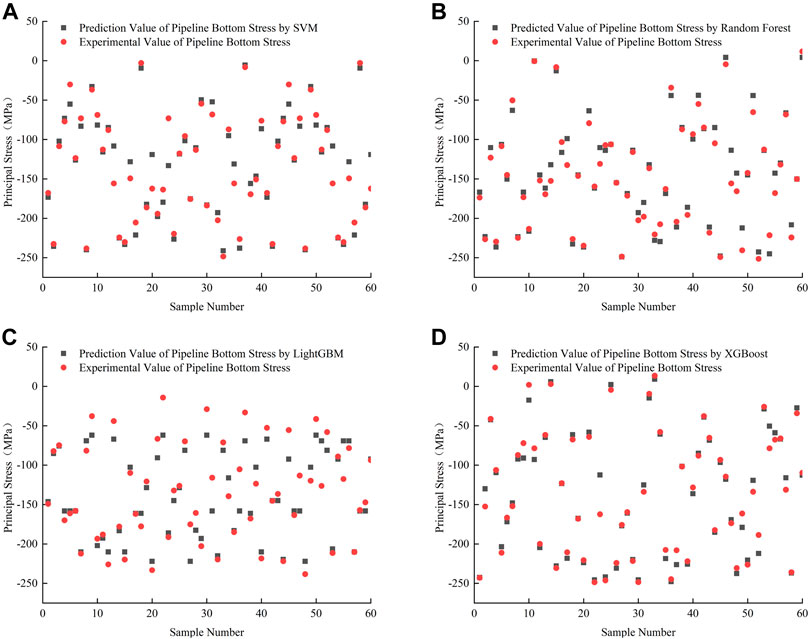
FIGURE 8. Regression verification of four algorithms [(A) SVM Regression; (B) Random Forest Regression; (C) LightGBM Regression; (D) XGBoost Regression].

FIGURE 9

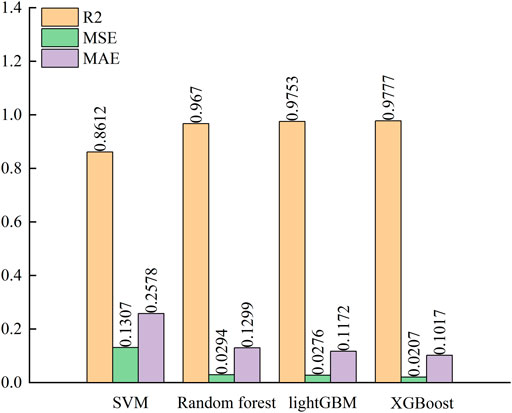
FIGURE 9. Histogram of evaluation indicators for four machine learning algorithms.

Pipeline Stress Prediction Under Freeze-Thaw Cycles Based on XGBoost

With an increase in the number of freeze-thaw cycles, the gravity and frost heaving force on the pipeline had coupled aggravated effect on the stressed state. However, when a certain number of freeze-thaw cycles was reached, this effect tended to be stable and saturated.

Twelve ML models were used to simulate 10–20 freeze-thaw cycles of the pipeline under study to verify the ratcheting effect further. Besides the proposed XGBoost model, these included Linear Regression, SVM, Random Forest, Gradient-Boosted Decision Trees (GBDT), LightGBM, BP Neural Network, Decision Tree, K-Nearest Neighbors (KNN), Adaboost, Extratrees, and Catboost models (Zhang Y. G. et al., 2021, 2021d; 2021e).

The prediction results on the principal stress evolution at the pipeline bottom are depicted in Figure 10.

FIGURE 10

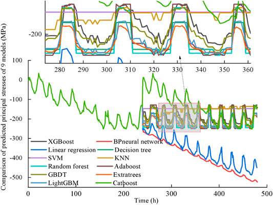
FIGURE 10. Principal stress evolutions at the pipeline bottom predicted by 12 ML models, with a partial enlargement.

As seen in Figure 10, the Q345 steel pipeline bottom stress predictions based on KNN, SVM, and Decision Tree were strongly inconsistent with the test results. For example, the stress predicted by the Decision Tree and SVM grew linearly with time, which was not consistent with the experimental pattern. However, the high stress predicted by KNN was concentrated in a small area, which could not guarantee pipeline safety.

It can be seen in Figure 10 that the Q345 pipeline stress evolutions predicted via the BP Neural Network, Linear Regression, and Catboost had a gradually increasing trend, which did not comply with the experimentally observed ratcheting effect. Therefore, these models had to be excluded as inapplicable ones. The curves established by Random Forest, Adaboost, and Extratrees are not time-sensitive and temperature-sensitive, so they were also excluded from further consideration. The stress predictions of the Q345 oil pipeline established by the XGBoost and LightGBM were both quite accurate, combining high correlation coefficients (R²) with small mean square errors (MSE) and mean absolute errors (MAE). The highest R² of XGBoost was 0.978, and the lowest MSE and MAE were 0.021 and 0.102, respectively. This implied that the XGBoost-based prediction model of the Q345 pipeline had high prediction accuracy, and the introduction of regularization parameters could effectively avoid overfitting.

As shown in Figure 11, the prediction data of the LightGBM model after 240 h poorly reflected the stress fluctuation at the bottom of the buried oil pipeline under the freeze-thaw cycling. Its time-temperature sensitivity was relatively low, but the model had high safety margins.

FIGURE 11

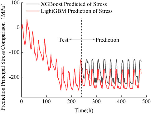
FIGURE 11. Prediction of the principal stress evolution at the pipeline bottom via XGBoost and LightGBM.

During 10–20 freeze-thaw cycles, the principal stress of the pipeline predicted via the XGBoost-based model fluctuated between -131.230 and -224.105 MPa, while the predicted and observed fluctuation patterns were very close.

As shown in Figure 12, during a freeze-thaw cycling process, the volumetric strain of the water-bearing frozen soil was relatively small, while the compressive stress at the pipeline bottom reached 69.785 MPa. Significant changes occurred only when the strain accumulation in the pipeline continued with each new cycle. After 13–14 freeze-thaw cycles, the maximum principal stress in the Q345 steel pipe tended to be saturated.

FIGURE 12

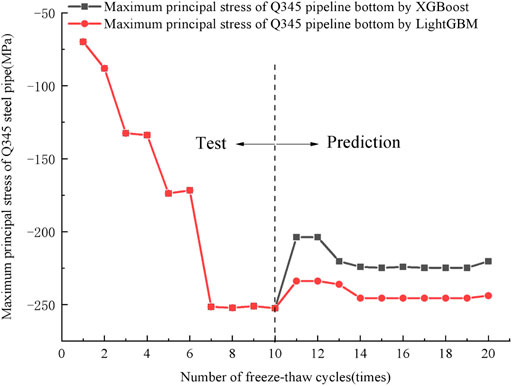
FIGURE 12. The maximum principal stress evolution at the pipeline bottom with the number of freeze-thaw cycles.

With the pursuit of a more reliable stress prediction in cold-region pipeline engineering, the LightGBM algorithm, which had higher safety margins than the XGBoost, could be alternatively used. However, its time and temperature sensitivities were unsatisfactory, therefore the high-precision XGBoost model should be used as the main one. Then, to increase the safety of pipe-soil interaction, the LightGBM can be used to predict the maximum stress in practical engineering to increase the safety margin of the XGBoost prediction results (Gao et al., 2020; Zhang X. et al., 2021, Zhang et al., 2021 Y., Zhang et al., 2022; Chelgani et al., 2021; Huang et al., 2021; Ma et al., 2021; Wang et al., 2021).

DISCUSSION ON THM COUPLING Under Freeze-Thaw Cycles

THM Coupling Mechanism

In rock and soil mechanics, multi-field coupling usually refers to the interaction between the seepage, temperature, and stress fields of rock and soil. The THM coupling mechanism and coupling equation of pipeline stress under freeze-thaw cycles are presented in Figure 13.

FIGURE 13

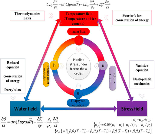
FIGURE 13. THM coupling mechanism and equation.

The stress evolution of buried oil pipelines under freeze-thaw cycles is closely related to the frozen soil’s moisture, temperature, and stress fields. Temperature gradient and soil water potential are the main driving forces for water migration. Moisture content and porosity are internal factors controlling water distribution. Therefore, the Richards equation with moisture content as a variable and phase transition account was applied. The transient heat conduction equation, which treated the volumetric strain effect as temperature variation, was established based on heat transfer theory and frozen soil mechanics.

According to Figures 3, 13, with the freezing and thawing cycles, the evolution law of principal stress at the top and bottom pipeline was consistent. Compared with the temperature time-history curve, the stress at the bottom pipeline had a lag. During the soil freezing process, the water in the soil was subjected to the combined action of pore stress and gravity. With the freezing and thawing cycles, the freezing edge of pore water pressure decreased, while the stress in the pipeline increased. After six freezing and thawing cycles, the pore water pressure was balanced, and the stress in the pipeline tended to be stable. Pipeline stress increased with temperature, while it dropped with increased temperature in the soil melting process. This implied that at a certain initial moisture content, the pipeline-soil force was affected by the pore water pressure, the number of freeze-thaw cycles, and the frost heaving force.

According to Figures 6, 13, due to the temperature gradient effect, the unfrozen water migrated to the soil surface at the beginning of the freeze-thaw cycles. Due to the in situ freezing of pore water, the pore pressure in the freezing edge increased sharply. When the pore pressure in frozen soil exceeded the soil separation stress, the soil was separated. An ice lens began to form, and water migration to the ice lens provided its continuous growth. As a result, the multilayer ice lens was formed, and the pipeline stress was accumulated. After six freeze-thaw cycles, when the initial moisture content exceeded 16%, a large frost heaving force between the pipe and soil was generated. The initial water content strongly related to the pipeline stress: the higher the former, the more significant the latter’s variation. At water contents exceeding 16%, the pipeline stress in the sixth freeze-thaw cycle decreased sharply. Therefore, the pipeline with high water content under multiple freeze-thaw cycles faced the risk of damage.

In summary, the pipe-soil interaction force was affected by initial moisture content, freeze-thaw cycles, frost heaving force, pore water pressure, temperature gradient, and other influencing factors.

Suggestions and Prospects

The temperature gradient changes and influence on frozen soil conditions must be considered. The simulated pipeline temperature was constant, ignoring the temperature change under permafrost conditions. Therefore, the oil temperature of the pipeline should be set as a step function in the subsequent research to simulate the actual pipeline operation.

Under THM coupling, pipeline stress accumulation is caused by frost heaving and thawing settlement. It can be used for pipeline design in seasonal frozen areas, but its physical mechanism has not been identified yet. The mechanical behavior of buried oil pipelines should be studied using comparative experimental research, theoretical research, numerical simulation, thermodynamics, and fluid mechanics.

The pipe-soil interaction process is also affected by the fluid in the pipe, temperature gradient, heat transfer, flow rate, particle size, and erosion-corrosion synergy. Under the action of erosion-corrosion, buried pipeline stress evolution is very complex. Therefore, the pipeline stress model should not only consider time-varying THM phenomena related to the constitutive behavior of frozen soil but also account for the interface deterioration of fluid and pipeline.

Conclusion

Using the background of the Da-Qing section of the China-Russia buried oil pipeline, this study optimized the freeze-thaw cycling test device based on the similarity theory. The general rule of pipeline stress evolution under freeze-thaw cycles was obtained. The COMSOL model verified the stress evolution of the pipeline under freeze-thaw cycles and predicted the stress evolution for different moisture contents. This verification realized the THM coupling of buried pipelines. The XGBoost-based prediction results made it possible to draw the following conclusions.

1) In a freeze-thaw process, the compressive stress at the pipeline bottom reached -69.785 MPa. The principal stress value increased gradually with the number of freeze-thaw cycles. After eight freeze-thaw cycles, the principal stress reached the extreme value of −252.437 MPa (i.e., 73.17% of yield stress). After fourteen freeze-thaw cycles, the principal compressive stress of the Q345 steel pipeline reached -224.733 MPa (65.14% of the yield stress) and tended to be saturated. This was consistent with the ratcheting effect predicted by the freeze-thaw cycle theory (Cherniavsky, 2018). Therefore, pipeline scale test had important reference value for actual pipeline engineering design.

2) Numerical simulation was performed to study the effect of initial moisture content (5, 10, 16, 20, 25, and 30%) on the pipe-soil interaction. The stress at the pipeline bottom increased with the moisture content w. However, this increase was the most obvious at w = 20–30%, indicating that at moisture contents below 16%, the number of freeze-thaw cycles had little effect on the frost heaving force of the frozen silty clay.

3) The principal stress prediction for the Q345 oil pipeline established via the XGBoost model was excellent, featuring R² = 0.978, MSE = 0.0207, MAE = 0.102, and RMSE = 11.0673. This result shows that the prediction accuracy of the Q345 pipeline prediction model was high. The XGBoost regression model established a nonlinear relationship between the test parameters and the pipeline stress, predicting the pipeline stress evolution for 10–20 freeze-thaw cycles.

4) Pursuing better stress prediction effects in pipeline engineering in cold regions, the tree algorithm combined with the XGBoost integration was introduced into the regular term parameters, effectively avoiding overfitting. The superposition of many decision trees improved the calculation accuracy, and the iteration efficiency was improved by the second-order Taylor expansion of the objective function. It could better meet the engineering requirements of the oil pipeline stress monitoring cycle, high precision, and large data volume.

5) Under 10–20 freeze-thaw cycles, the principal stress of the pipeline predicted by the XGBoost model fluctuated from −31.235 to −224.105 MPa, which results were consistent with the experimental ones.

Data Availability Statement

The original contributions presented in the study are included in the article/Supplementary Material, further inquiries can be directed to the corresponding author.

Author Contributions

Z-CT: Experimental design Y-CT, BL, X-YL, YL: Data analysis Y-CT, BL, X-YL, YL, and Y-DZ: Instrument operation Y-CT: Provide the whole idea.

Funding

This research was funded by the National Natural Science Foundation of China under grant No. 52076036.

Conflict of Interest

The authors declare that the research was conducted in the absence of any commercial or financial relationships that could be construed as a potential conflict of interest.

Publisher’s Note

All claims expressed in this article are solely those of the authors and do not necessarily represent those of their affiliated organizations, or those of the publisher, the editors and the reviewers. Any product that may be evaluated in this article, or claim that may be made by its manufacturer, is not guaranteed or endorsed by the publisher.

Acknowledgments

The authors gratefully acknowledge the financial support of this study by the National Natural Science Foundation of China (Grant No. 52076036).

Supplementary Material

The Supplementary Material for this article can be found online at: https://www.frontiersin.org/articles/10.3389/feart.2022.839549/full#supplementary-material

References

Abbasi, R. A., Javaid, N., Ghuman, M. N. J., Khan, Z. A., and Ur Rehman, S. (2019). “Short Term Load Forecasting Using XGBoost,” in Workshops of the International Conference on Advanced Information Networking and Applications (Cham: Springer), 1120–1131. doi:10.1007/978-3-030-15035-8_108

CrossRef Full Text | Google Scholar

Andersland, O. B., and Ladanyi, B. (2003). Frozen Ground Engineering. John Wiley & Sons.

Google Scholar

Bekele, Y. W., Kyokawa, H., Kvarving, A. M., Kvamsdal, T., and Nordal, S. (2017). Isogeometric Analysis of THM Coupled Processes in Ground Freezing. Comput. Geotechnics 88, 129–145. doi:10.1016/j.compgeo.2017.02.020

CrossRef Full Text | Google Scholar

Boguchevskaya, E. M., Dimov, I. L., and Dimov, L. A. (2016). Determining Tilt in Tanks Used to Store Oil and Oil Products during Hydraulic Testing and Operation. Soil Mech. Found. Eng. 53 (1), 35–38. doi:10.1007/s11204-016-9361-0

CrossRef Full Text | Google Scholar

Carlson, L. E., and Nixon, J. F. (1988). Subsoil Investigation of Ice Lensing at the Calgary, Canada, Frost Heave Test Facility. Can. Geotechnical J. 25 (2), 307–319. doi:10.1139/t88-033

CrossRef Full Text | Google Scholar

Chelgani, S. C., Nasiri, H., and Alidokht, M. (2021). Interpretable Modeling of Metallurgical Responses for an Industrial Coal Column Flotation Circuit by XGBoost and SHAP-A “Conscious-lab” Development. Int. J. Mining Sci. Technology. doi:10.1016/j.ijmst.2021.10.006

CrossRef Full Text | Google Scholar

Chen, T., and Guestrin, C. (2016). “Xgboost: A Scalable Tree Boosting System,” in Proc. 22nd ACM SIGKDD Int. Conf. On Knowledge Discovery and Data Mining, SanFrancisco, California, USA, Association for Computing Machinery, 785–794. doi:10.1145/2939672.2939785

CrossRef Full Text | Google Scholar

Cherniavsky, A. (2018). Ratcheting Analysis of "Pipe-Freezing Soil" Interaction. Cold Regions Sci. Technology 153, 97–100. doi:10.1016/j.coldregions.2018.05.005

CrossRef Full Text | Google Scholar

Dong, W., Huang, Y., Lehane, B., and Ma, G. (2020). XGBoost Algorithm-Based Prediction of concrete Electrical Resistivity for Structural Health Monitoring. Automation in Construction 114, 103155. doi:10.1016/j.autcon.2020.103155

CrossRef Full Text | Google Scholar

Dvoskina, S. N., Vershinin, V. V., Emelyanov, T. A., and Markov, V. N. (2015). Possibility of Peat Industry’s Experience Usage during Oil Pipe-Laying on Swamps. Ecol. Industry Russia 8, 47–48. doi:10.18412/1816-0395-2013-8-47-48

CrossRef Full Text | Google Scholar

Fuschi, P., Pisano, A. A., and Weichert, D. (2015). Direct Methods for Limit and Shakedown Analysis of Structures. Berlin: Springer.

Google Scholar

Gao, L., Gao, F., Zhang, Z., and Xing, Y. (2020). Research on the Energy Evolution Characteristics and the Failure Intensity of Rocks. Int. J. Mining Sci. Technology 30 (5), 705–713. doi:10.1016/j.ijmst.2020.06.006

CrossRef Full Text | Google Scholar

Gokhfeld, D. A., and Charniavsky, O. F. (1980). “Limit Analysis of Structures at thermal Cycling,” in Springer Science & Business Media, Alphen aan den Rijn, Sijthoff & Noordhoff 1980, XXVIII, 537 S., ISBN 90-286-0455-3. ZAMM - Journal of Applied Mathematics and Mechanics / Zeitschrift fûr Angewandte Mathematik und Mechanik 64(8), 422–423. doi:10.1002/zamm.19820620823

CrossRef Full Text | Google Scholar

Guo, X. F., Xia, Z. Z., Wu, J. Y., and Wang, R. Z. (2010). Numerical Analysis and Similarity experiment on Temperature Field of Underground Pipe. Acta Energiae Solaris Sinica 31 (6), 727–731. Available at:https://CNKISUN:TYLX.0.2010-06-016.

CrossRef Full Text | Google Scholar

Haxaire, A., Aukenthaler, M., and Brinkgreve, R. B. J. (2017). Application of a Thermo-Hydro-Mechanical Model for Freezing and Thawing. Proced. Eng. 191, 74–81. doi:10.1016/j.proeng.2017.05.156

CrossRef Full Text | Google Scholar

Huang, S., He, Y., Yu, S., and Cai, C. (2021). Experimental Investigation and Prediction Model for UCS Loss of Unsaturated Sandstones under Freeze-Thaw Action. Int. J. Mining Sci. Technology. doi:10.1016/j.ijmst.2021.10.012

CrossRef Full Text | Google Scholar

Huang, S. L., Bray, M. T., Akagawa, S., and Fukuda, M. (2004). Field Investigation of Soil Heave by a Large Diameter Chilled Gas Pipeline experiment, Fairbanks, Alaska. J. cold regions Eng. 18 (1), 2–34. doi:10.1061/(ASCE)0887-381X(2004)18:1(2)

CrossRef Full Text | Google Scholar

Huang, S. L., Yang, K., Akagawa, S., Fukuda, M., and Kanie, S. (2015). “Frost Heave Induced Pipe Strain of an Experimental Chilled Gas Pipeline.,” in Innovative Materials and Design for Sustainable Transportation Infrastructure, Fairbanks, Alaska, International Symposium on Systematic Approaches to Environmental Sustainability in Transportation, 405–416. doi:10.1061/9780784479278.037

CrossRef Full Text | Google Scholar

Jin, H., Hao, J., Chang, X., Zhang, J., Qi, J., Lü, L., et al. (2010). Zonation and Assessment of Frozen-Ground Conditions for Engineering Geology along the China-Russia Crude Oil Pipeline Route from Mo'he to Daqing, Northeastern China. Cold Regions Sci. Technology 64 (3), 213–225. doi:10.1016/j.coldregions.2009.12.003

CrossRef Full Text | Google Scholar

Kang, J. Y., Park, D. H., and Lee, J. (2016). Effect of Freezing Saturated sandy Soil under Undrained Condition on a Buried Steel Pipe. Int. J. Control. Automation 9 (5), 297–306. doi:10.14257/ijca.2016.9.5.29

CrossRef Full Text | Google Scholar

Kim, J., Lee, H., and Oh, J. (2020). Study on Prediction of Ship's Power Using Light GBM and XGBoost. JAMET 44 (2), 174–180. doi:10.5916/jamet.2020.44.2.174

CrossRef Full Text | Google Scholar

Kim, K., Zhou, W., and Huang, S. L. (2008). Frost Heave Predictions of Buried Chilled Gas Pipelines with the Effect of Permafrost. Cold Regions Sci. Technology 53 (3), 382–396. doi:10.1016/j.coldregions.2008.01.002

CrossRef Full Text | Google Scholar

Li, G., Sheng, Y., Jin, H., Ma, W., Qi, J., Wen, Z., et al. (2010). Development of Freezing-Thawing Processes of Foundation Soils Surrounding the China-Russia Crude Oil Pipeline in the Permafrost Areas under a Warming Climate. Cold Regions Sci. Technology 64 (3), 226–234. doi:10.1016/j.coldregions.2009.08.006

CrossRef Full Text | Google Scholar

Li, H., Lai, Y., Wang, L., Yang, X., Jiang, N., Li, L., et al. (2019). Review of State of the Art: Interactions between a Buried Pipeline and Frozen Soil. Cold Regions Sci. Technology 157, 171–186. doi:10.1016/j.coldregions.2018.10.014

CrossRef Full Text | Google Scholar

Liu, W. B., Yu, W. B., Yi, X., and Chen, L. (2014). Heat Effect Analysis of Buried Oil Pipeline in the Qinghai-Tibet Plateau. Appl. Mech. Mater.501, 211–217. Trans Tech Publications Ltd.10.4028/. doi:10.4028/www.scientific.net/amm.501-504.211

CrossRef Full Text | Google Scholar

Ma, J., Li, X., Wang, J., Tao, Z., Zuo, T., Li, Q., et al. (2021). Experimental Study on Vibration Reduction Technology of Hole-By-Hole Presplitting Blasting. Geofluids. vol. 2021, Article ID 5403969, 10 pages. doi:10.1155/2021/5403969

CrossRef Full Text | Google Scholar

Mukhametdinov, H. K. (1996). The Device of Fastening of the Pipeline from the Ascent - the Patent for Invention RUS 2062938.

Google Scholar

Nishimura, S., Gens, A., Olivella, S., and Jardine, R. J. (2009). THM-coupled Finite Element Analysis of Frozen Soil: Formulation and Application. Géotechnique 59 (3), 159–171. doi:10.1680/geot.2009.59.3.159

CrossRef Full Text | Google Scholar

Nixon, M., Saiyar, M., Becker, D., and Pinkert, S. (2016). “Pipeline Uplift Resistance in Frozen Soil–Numerical Study,” in GeoVancouver at Vancouver CB (Canada.

Google Scholar

Prayogo, D., Cheng, M. Y., Wu, Y. W., and Tran, D. H. (2020). Combining Machine Learning Models via Adaptive Ensemble Weighting for Prediction of Shear Capacity of Reinforced-concrete Deep Beams. Eng. Comput. 36 (3), 1135–1153. doi:10.1007/s00366-019-00753-w

CrossRef Full Text | Google Scholar

Slusarchuk, W. A., Clark, J. I., Nixon, J. F., Morgenstern, N. R., and Gaskin, P. N. (1978). Field Test Results of a Chilled Pipeline Buried in Unfrozen Ground. In Proc. 3rd Int. Conf. On Permafrost. Edmonton 1, 878–883. doi:10.1016/0148-9062(80)90323-x

CrossRef Full Text | Google Scholar

Su, H., Wen, Z., Wang, F., and Hu, J. (2016). Dam Structural Behavior Identification and Prediction by Using Variable Dimension Fractal Model and Iterated Function System. Appl. Soft Comput. 48, 612–620. doi:10.1016/j.asoc.2016.07.044

CrossRef Full Text | Google Scholar

Teng, Z. C., Liu, X. Y., Liu, Y., Zhao, Y. X., Liu, K. Q., and Teng, Y. C. (2021). Stress-strain Assessments for Buried Oil Pipelines under Freeze-Thaw Cyclic Conditions. J. Press. Vessel Technology 143 (4), 041803. doi:10.1115/1.4049712

CrossRef Full Text | Google Scholar

Wang, J., Zuo, T., Li, X., Tao, Z., and Ma, J. (2021). Study on the Fractal Characteristics of the Pomegranate Biotite Schist under Impact Loading. Geofluids 2021. doi:10.1155/2021/1570160

CrossRef Full Text | Google Scholar

Wen, Z., Sheng, Y., Jin, H., Li, S., Li, G., and Niu, Y. (2010). Thermal Elasto-Plastic Computation Model for a Buried Oil Pipeline in Frozen Ground. Cold Regions Sci. Technology 64 (3), 248–255. doi:10.1016/j.coldregions.2010.01.009

CrossRef Full Text | Google Scholar

Wu, Y., Sheng, Y., Wang, Y., Jin, H., and Chen, W. (2010). Stresses and Deformations in a Buried Oil Pipeline Subject to Differential Frost Heave in Permafrost Regions. Cold regions Sci. Technol. 64 (3), 256–261. doi:10.1016/j.coldregions.2010.07.004

CrossRef Full Text | Google Scholar

Xu, G., Qi, J., and Jin, H. (2010). Model Test Study on Influence of Freezing and Thawing on the Crude Oil Pipeline in Cold Regions. Cold Regions Sci. Technology 64 (3), 262–270. doi:10.1016/j.coldregions.2010.04.010

CrossRef Full Text | Google Scholar

Xu, R., Su, H. Z., and Yang, L. F. (2021). Dam Deformation Prediction Model Based on GP-XGBoost. Adv. Sci. Technology Water Resour. 41 (05), 41–46+70. Available at: https://kns.cnki.net/kcms/detail/32.1439.TV.2021 0917.1739.004.html. doi:10.3880/j.issn.1006-7647.2021.05.007

CrossRef Full Text | Google Scholar

Zhang, Chen. (2017). Medium-thick Plate Stress Analysis FeaturcExtraction and Defect Prediction Based on Genetic Algorithm. Ph.D. Dissertation. Northeastern University. SHE, 2017. (in Chinese) https://kns.cnki.net/KCMS/detail/detail.aspx?dbname=CMFD201901&filename=1019031131.nh.

Google Scholar

Zhang, H. X. (2006). Strain Measurement and Data Processing Method in Complex Stress State. China Meas. Test 03.32 (2), 52–55. doi:10.3969/j.issn.1674-5124.2006.02.017

CrossRef Full Text | Google Scholar

Zhang, H., Zhi, B., Liu, E., and Wang, T. (2020a). Study on Varying Characteristics of Temperature Field and Moisture Field of Shallow Loess in the Freeze-Thaw Period. Adv. Mater. Sci. Eng. 2020. doi:10.1155/2020/1690406

CrossRef Full Text | Google Scholar

Zhang, T., Yu, L., Su, H., Zhang, Q., and Chai, S. (2021b). Experimental and Numerical Investigations on the Tensile Mechanical Behavior of Marbles Containing Dynamic Damage. International Journal of Mining Science and Technology. 32 (1), 89–102. doi:10.1016/j.ijmst.2021.08.002

CrossRef Full Text | Google Scholar

Zhang, X., Wu, Y., Zhai, E., and Ye, P. (2021a). Coupling Analysis of the Heat-Water Dynamics and Frozen Depth in a Seasonally Frozen Zone. J. Hydrol. 593, 125603. doi:10.1016/j.jhydrol.2020.125603

CrossRef Full Text | Google Scholar

Zhang, Y. G., Xie, Y. L., Zhang, Y., Qiu, J. B., and Wu, S. X. (2021c). The Adoption of Deep Neural Network (DNN) to the Prediction of Soil Liquefaction Based on Shear Wave Velocity. Bull. Eng. Geology. Environ. 80 (6), 5033–5060. doi:10.1007/s10064-021-02250-1

CrossRef Full Text | Google Scholar

Zhang, Y. G., Tang, J., Cheng, Y., Huang, L., Guo, F., Yin, X., et al. (2022). Prediction of Landslide Displacement with Dynamic Features Using Intelligent Approaches. Int. J. Mining Sci. Technology 12 (1), 368–382. doi:10.1016/j.ijmst.2022.02.004

CrossRef Full Text | Google Scholar

Zhang, Y. G., Tang, J., He, Z. Y., Tan, J., and Li, C. (2021e). A Novel Displacement Prediction Method Using Gated Recurrent Unit Model with Time Series Analysis in the Erdaohe Landslide. Nat. Hazards 105 (1), 783–813. doi:10.1007/s11069-020-04337-6

CrossRef Full Text | Google Scholar

Zhang, Y. G., Tang, J., Liao, R. P., Zhang, M. F., Zhang, Y., Wang, X. M., et al. (2021d). Application of an Enhanced BP Neural Network Model with Water Cycle Algorithm on Landslide Prediction. Stochastic Environ. Res. Risk Assess. 35 (61-65), 1–19. doi:10.1007/s00477-020-01920-y

CrossRef Full Text | Google Scholar

Zhang, Y., and Michalowski, R. L. (2015). Thermal-hydro-mechanical Analysis of Frost Heave and Thaw Settlement. J. Geotechnical Geoenvironmental Eng. 141 (7), 04015027. doi:10.1061/(ASCE)GT.1943-5606.0001305

CrossRef Full Text | Google Scholar

Zhang, Y., Qiu, J., Zhang, Y., and Xie, Y. (2021f). The Adoption of a Support Vector Machine Optimized by GWO to the Prediction of Soil Liquefaction. Environ. Earth Sci. 80 (9), 1–9. doi:10.1007/s12665-021-09648-w

CrossRef Full Text | Google Scholar